The focus:
The basics of multitasking in microcontroller projects, characterized by contrl loops, interrupt service routines (ISRs) ansd switching from task to task.

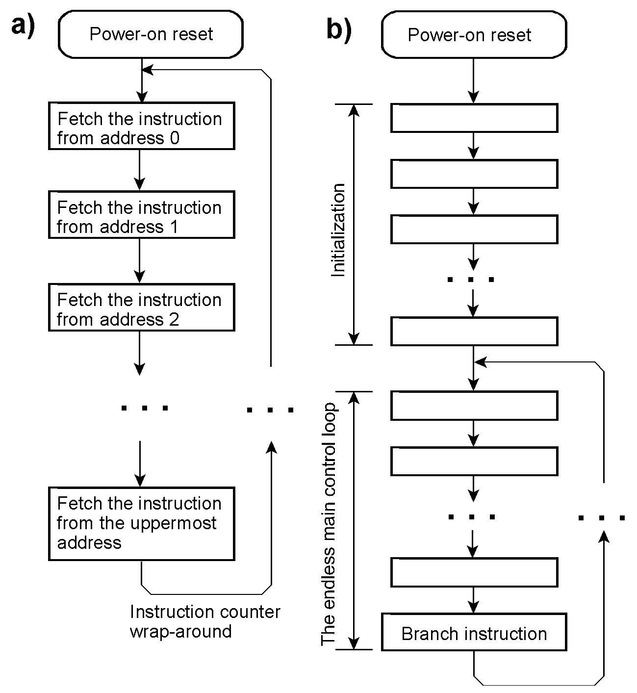
Electronic data processing – the fundamental paradigm           
Electronic data processing generates results from input and stored data that are output or stored.  A typical EDP program corresponds to the scheme input – process – output

Figure 1
Electronic data processing (EDP). a) shows the most general scheme. One of the most essential tenets of EDP, however, is that data are not only fetched from outside and results are not only emitted, but that data are stored internally as well. Hence, it is appropriate to highlight this feature even in the most basic block diagram, as shown in (b). c) illustrates the principal program flow.

Today’s microcontrollers and general-purpose processors are still EDP machines. Once switched on and initially reset, they fetch instruction after instruction out of the memory and execute them. If no branch instruction is included, the instruction counter will sometimes reach the uppermost memory address and wrap around to address zero (a). Consequently, each program must become an endless loop (b).

Figure 2
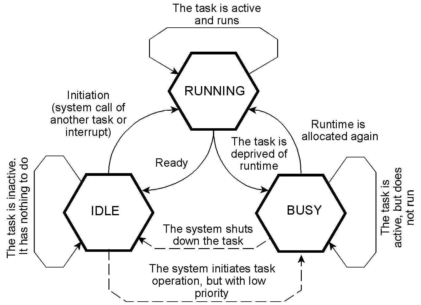
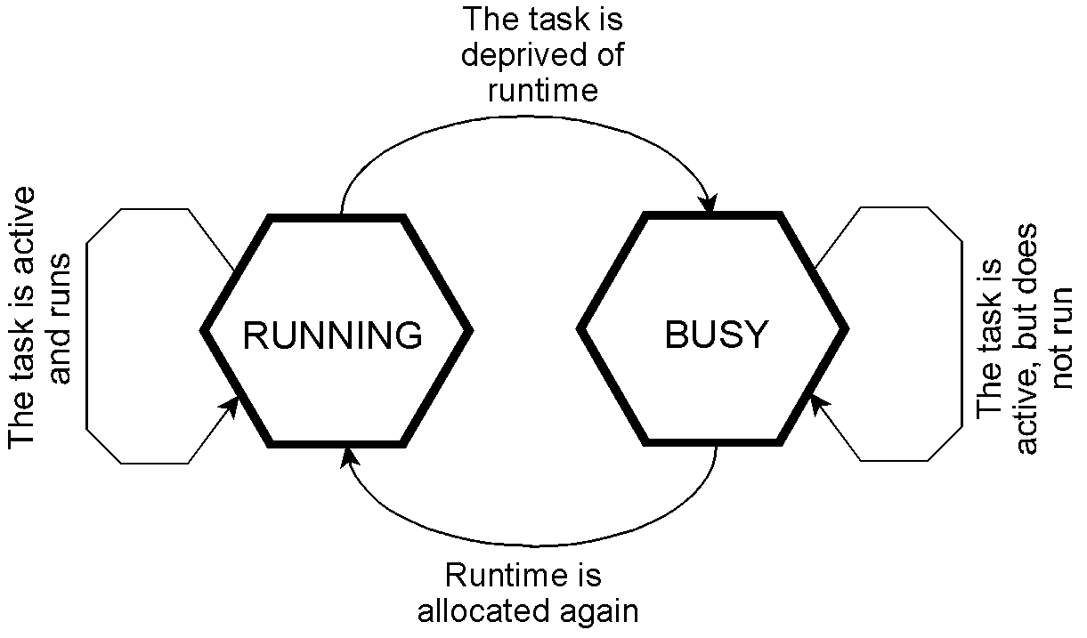
How a conventional processor works. Instruction address counting has not altered since the very beginning

By the way, I have occasionally used the processor behavior shown in (a)  for diagnostic purposes. In the appropriate diagnostic mode, an NOP instruction was forced onto the data bus. So, all address lines and some of the address decoding could be traced by an oscilloscope.

Multitasking means running multiple programs piecemeal simultaneously in a time-multiplexed fashion. This can be done only by querying in endless loops and by triggering interrupts. Here, we limit ourselves to basic, easy-to-comprehend principles of operation.

Tasks are comparatively small, not overly complex programs. Their runtime environments are called partitions. They are, so to speak, prefabricated areas in the memory, tailored to the demands of the particular tasks.

Princial task state models
 On a single processor, only one task can run at a time. Other tasks may be completely inactive or idle, others may be active or busy, that is, ready to run, provided they are given the opportunity. Thus, the tasks are distinguished by their state.

Here, we will discuss only straightforward state models that are appropriate for small microcontroller projects without advanced operating systems. The following state diagrams illustrate states and state transitions of a single task, regardless of how the transitions are triggered, be it by programmed branching, by system calls, or by interrupts.

Figure 2 shows all the states a task can enter. In the idle state, it is inactive, has nothing to do, and will not claim runtime.  In the running state, it is active and runs on the processor. When it is deprived of runtime, while still active, it transitions to the busy state, awaiting a new opportunity to proceed.

The task can command a state transition only if it is running. All other state transitions must be caused from the outside. Only an interrupt or a system call from another task may awaken the task out of the idle state and make it run. Only a running task may make itself idle, for example, by a READY system call, as depicted here. A more advanced system may cancel a task's operation by changing its state from busy to idle. Conversely, it may activate the task by making it busy, so it can participate in runtime allocation.

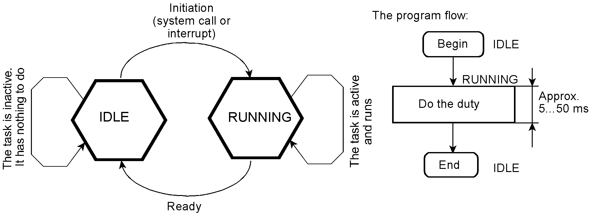
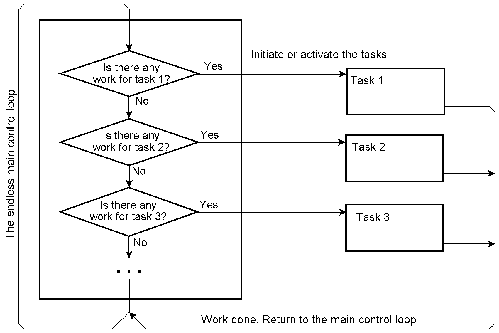
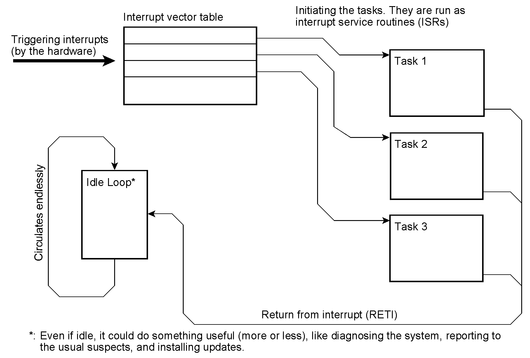
Figure 3
The three states a straightforward task can be in.

The state model can be simplified by omitting one of the states. According to Figure 4, the task has no busy state. To perform a particular action, it must be awakened from the idle state. When it has done its duty, it becomes idle again. This state model is adequate if the tasks are only short programs that always come to an end, say, after a few milliseconds. They do not need so much runtime that it must be shared between the tasks, and hence allocated. On the other hand, some provisions outside of those tasks are required to initiate them. It could be done by an endless main control loop or by interrupts.

Figure 4
The first simplified state model. The tasks run only on demand. It could be dubbed a start-stop operation.

To be able to do something, a program must run. The state model of shown above requires endlessly running programs outside the tasks or interrupt provisions that initiate all the task operations.  An alternative idea is to let all tasks run endlessly, so they can manage themselves. The only provision outside is a timer-based interrupt. Figure 5 shows the appropriate state model. From the beginning, that is, after power-on reset and initialization, all tasks are running in endless loops. They could be thought of as being executed in virtual machines, each with its own main control loop. The state transitions are only caused by the timer-based interrupts.

Figure 5
The alternative simplified state model. All tasks run endlessly. Timer-based interrupts provide each task with slices of runtime. The tasks could be thought of as running in virtual machines.

Each of the two-state models has its pros and cons (Table 1). Thus, the choice depends on the application requirements and the hardware platform.

Table 1
The simplified state models compared.

Some typical patterns of control loops
 The  next figures  are thought to illustrate principles of how control loops, tasks, and interrupt service routines could work together.

Figure 6
A generalized scheme of a main control loop that queries what to do and provides the tasks with work. In detail, however, it is not as simple as shown here, especially if a more complex state model (as depicted in Figure 3) is to be supported. Here, we are already on the way to a true real-time operating system.

Figure 7
The main control loop is divided into sections, each concerned with a particular task.  If the programs that treat the requests come to an end after a few milliseconds, it will fit well with the state model of Figure 4.

Figure 8
The tasks are activated solely by interrupts.  The main control loop shrinks to an idle loop. The task’s state model corresponds to Figure 4.

Figure 9
More demanding projects require interrupt service routines (ISRs) as well as tasks that are activated by the main control loop.

Invoking hard endless loops
Hard endless loops are programs that must be executed cyclically, regardless of which program sections are passed through.  This can be enforced by cooperative programming or by preempting via timer-initiated interrupts (Figure 10).

Figure 10
Hard endless loops may be called as subroutines (a) or enforced cyclically as interrupt service routines (b).

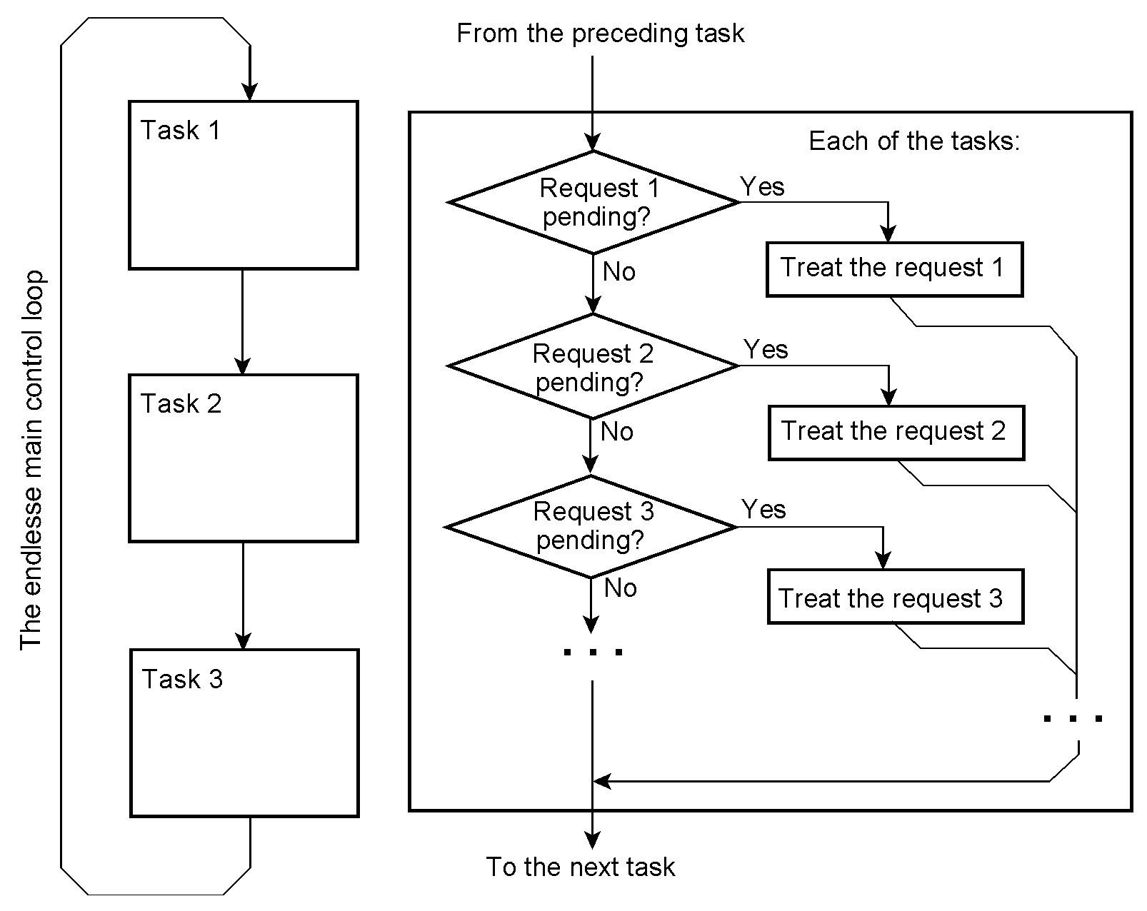
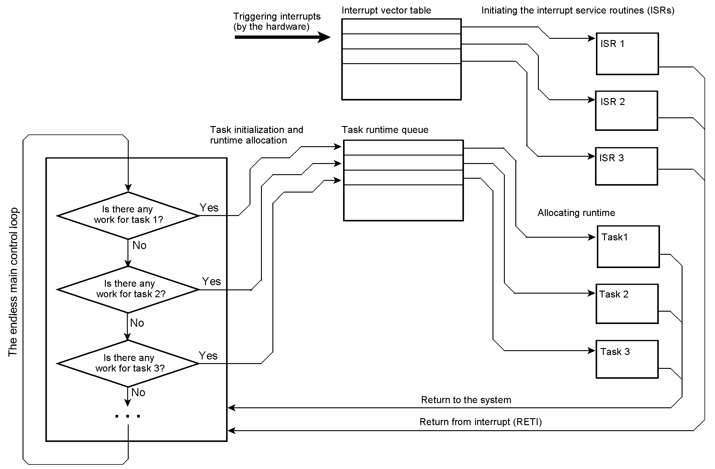
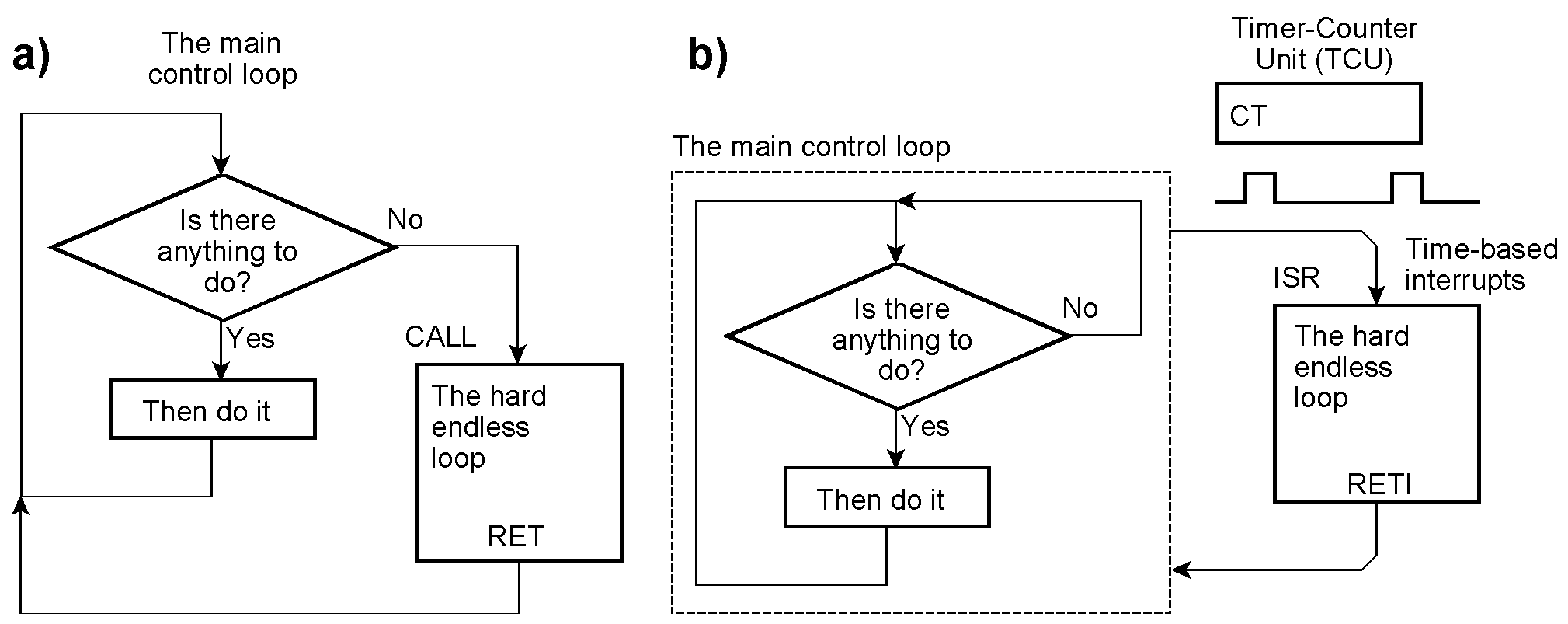
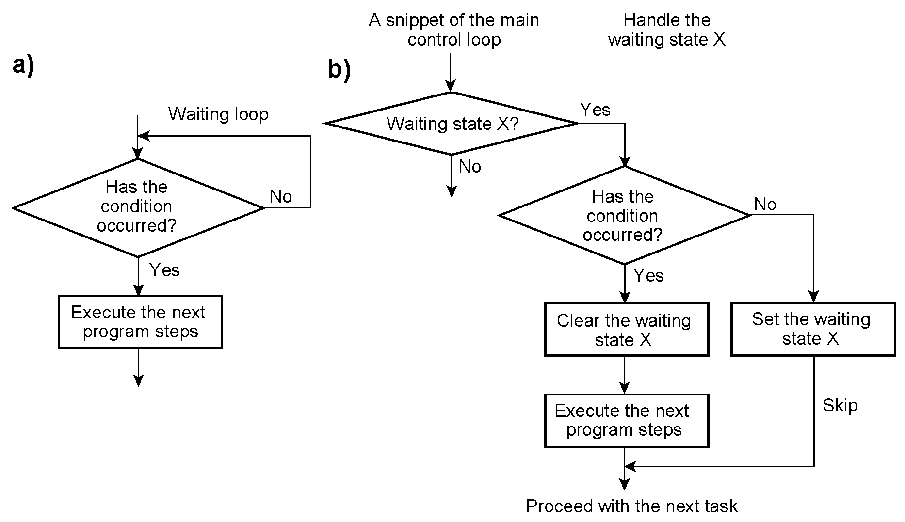
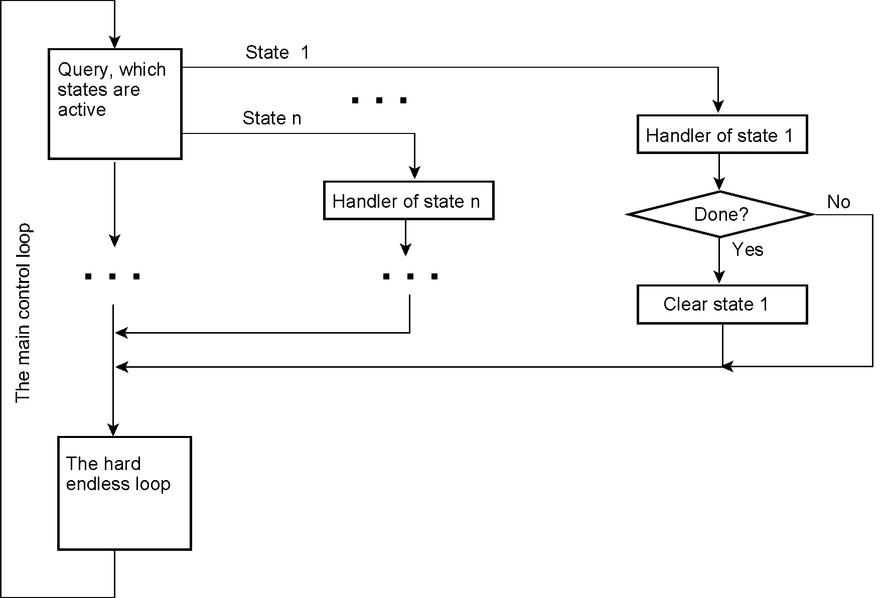
Implementing the hard endless loop as an interrupt service routine (ISR) is straightforward. Say you need 20 passes per second, then initialize a timer-counter unit (TCU) of your microcontroller to trigger an interrupt every 50 milliseconds.

It could, however, happen that the interrupt occurs, with respect to other activities, at an inappropriate time, or that the ISR eats up too much runtime, which is momentarily not acceptable.

Of course, with a powerful processor and an appropriate RTOS, such problems could be solved as a matter of routine. But here we talk about small microcontrollers and low-footprint programs.  

Alternatively, you may resort to cooperative multitasking. This way, you have the runtime allocation completely under program control (it is the same principle as implemented in Windows 3.x and the first Macs, but considerably more simplified). Here, too, however, are chances to commit annoying mistakes. In Figure 9 of the printed article, we have sketched the most basic approach to cooperative multitasking: to insert the hard endless loop (as a subroutine) into each waiting loop. Sometimes, that may work flawlessly. On the other hand, the inserted subroutine may consume scarce runtime that would be better spent running other tasks. In other words, it could be called more often than necessary.

When waiting loops eat up precious runtime, you must not program as shown in Figure 9 mentioned above or in Figure 11a below. If the waiting condition is not met, the other tasks must be given sufficient runtime. It could be done by dividing the application program into states and state handlers.

This is illustrated in Figure 11b by the example of a waiting state X. Instead of circulation in the waiting loop, as shown in Figure 11a, and thus wasting runtime, the application program established a waiting state (as an additional program variable). If the condition to be expected has occurred, the waiting state is cleared, and the program proceeds with the next step. Otherwise, the waiting state is retained, and the next program step is skipped.

Figure 12 depicts how the states, their handlers, the hard endless loop and the main control loop may fit together. Here, the hard endless loop is passed as a part of the main control loop, thus no runtime is wasted. The main control loop could even decide after how many passes the hard endless loop needs to be called. Waiting and other time-consuming activities are called via states. Within the state handlers, waiting loops are not permitted.

Figure 11
Two program snippets. (a) illustrates a programming habit to avoid if other tasks also need runtime. According to (b), the program memorizes, by a wait state variable, that it has to query a waiting condition. If the condition has not occurred yet, the next task gets runtime.

Figure 12
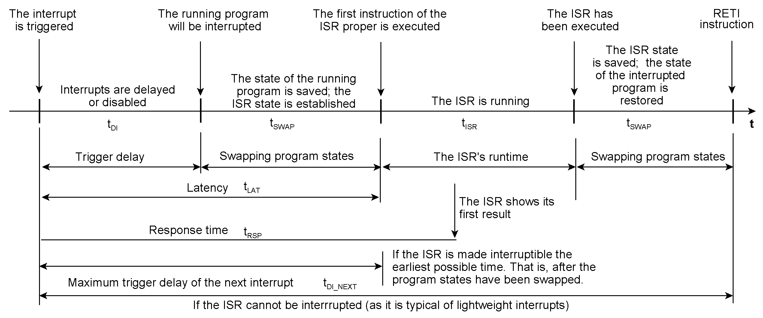
A sketch of the overall program organization centered around the main control loop.

The timing budget of an interrupt service routine (ISR)
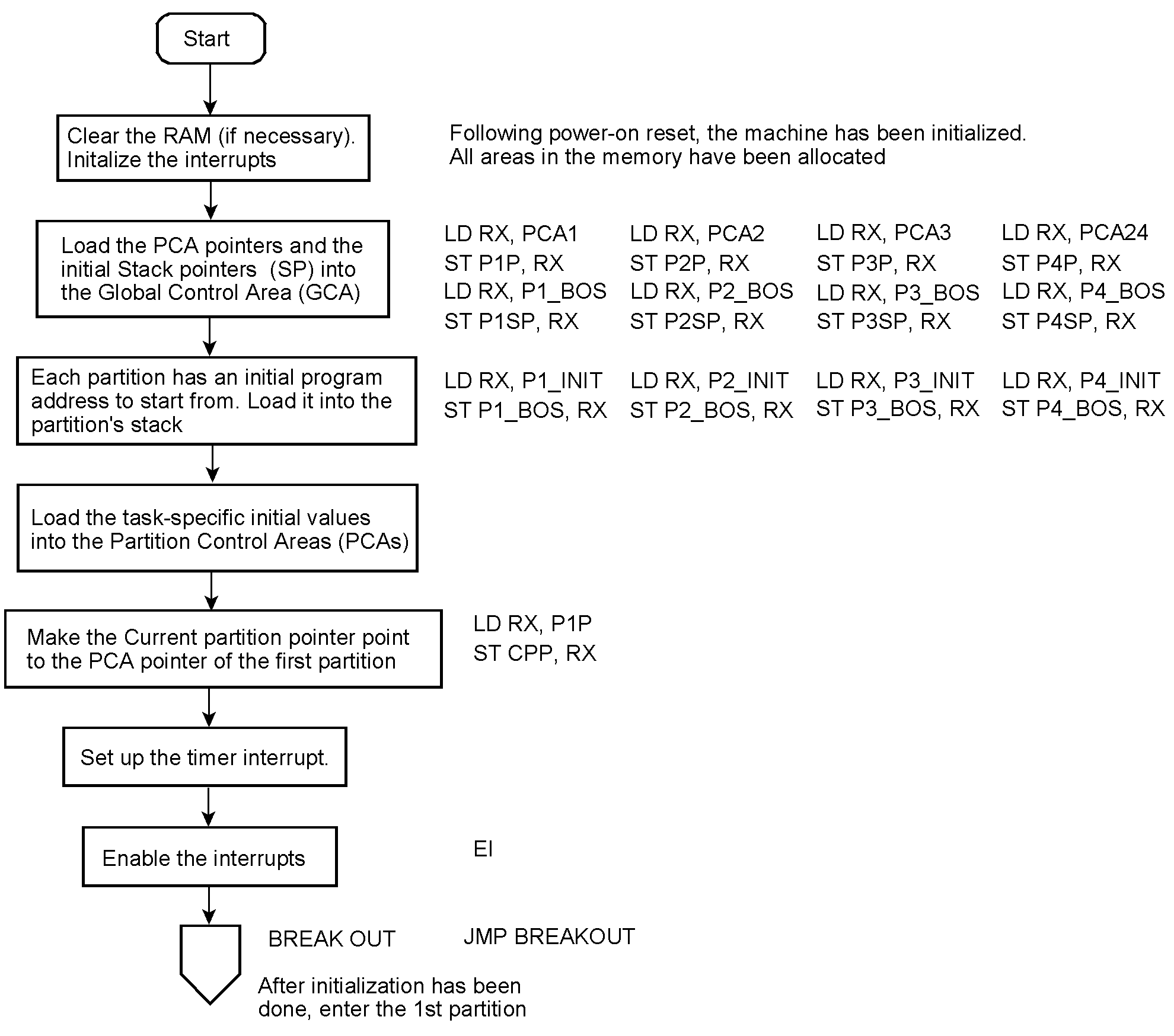
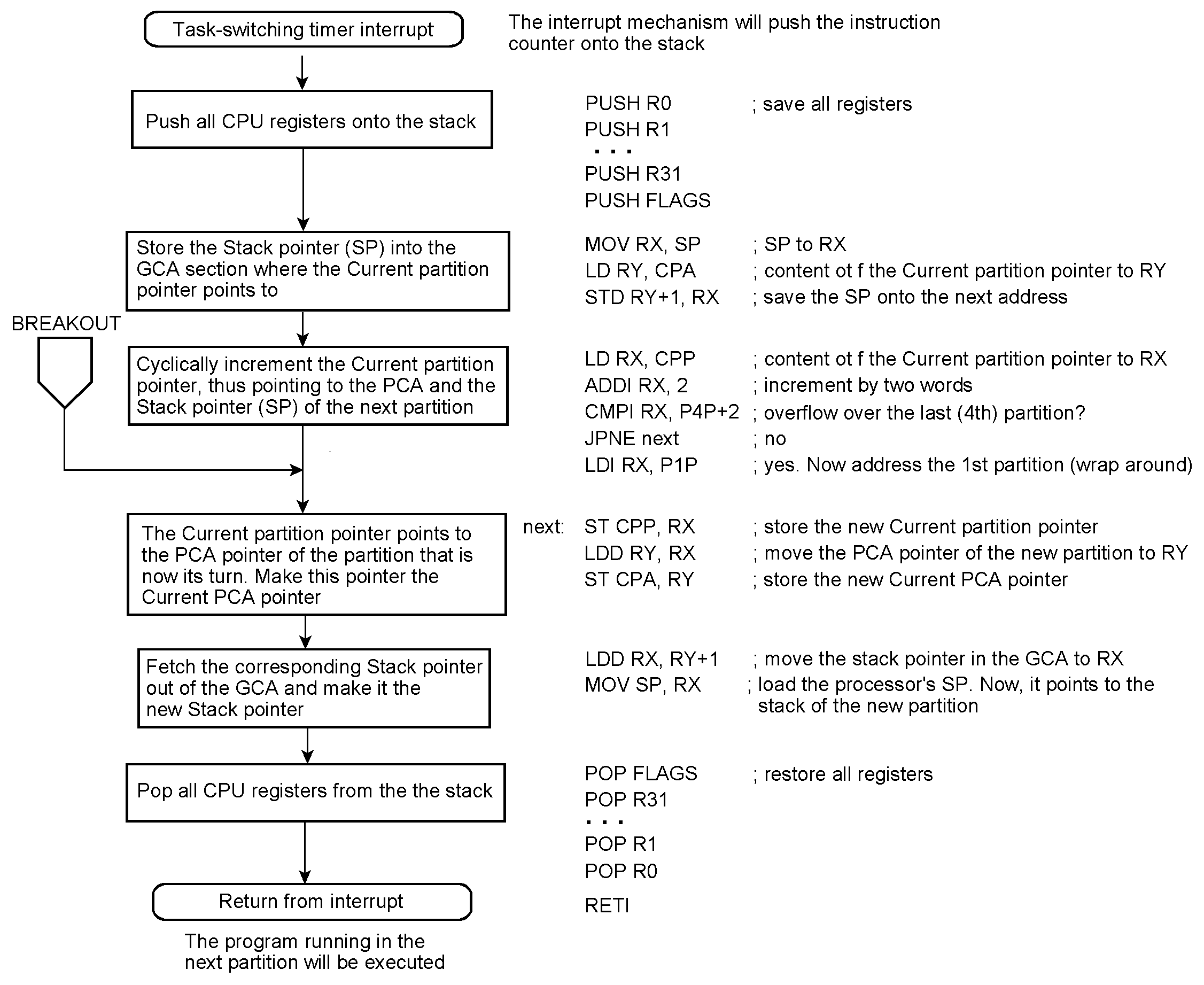
 In the printed article, we have explained the terms latency and respnose time. Here, Figure 13 supplements Figure 4 of the printed article.

Figure 13
The timing budget of an interrupt service routine (ISR) is shown in more detail.

Straightforward virtual machines by time slicing
 Figure 14 supplements Figure 14 in the printed article, showing the principal memory allocation im more detail. Figure 15 supplements Figure 15 in the printed text, showing a partition’s stack frame related to the AVR architecture. Figure 16 of the printed text has been dissected into Figures 16 and 17. The instructions are a pseudo-code, applicable to most accumulator and general-purpose register architectures.

RX designates the accumulator. RY designates a base address or index register. SP is the stack pointer. PUSH, POP, MOV, LD, ST, JMP, JPNE have their usual meanings. The first parameter is the destination.

STD = Store indirect with displacement.

Syntax: STD index register+displacement, data register.

LDD = Load indirect with displacement.

Syntax: LDD data register, index register+displacement, data register.

ADDI = Add an immediate value.

Syntax: ADDI data register, immediate value

LDI = Load an immediate value.

Syntax: LDI data register, immediate value.

CMPI = Compare with an immediate value.

Syntax: CMPI data register, immediate value.

Figure 14
The principal memory allocation.

Figure 15
The stack frame of an AVR microcontroller.

Figure 16
Initialization of time-slicing operation.

Figure 17
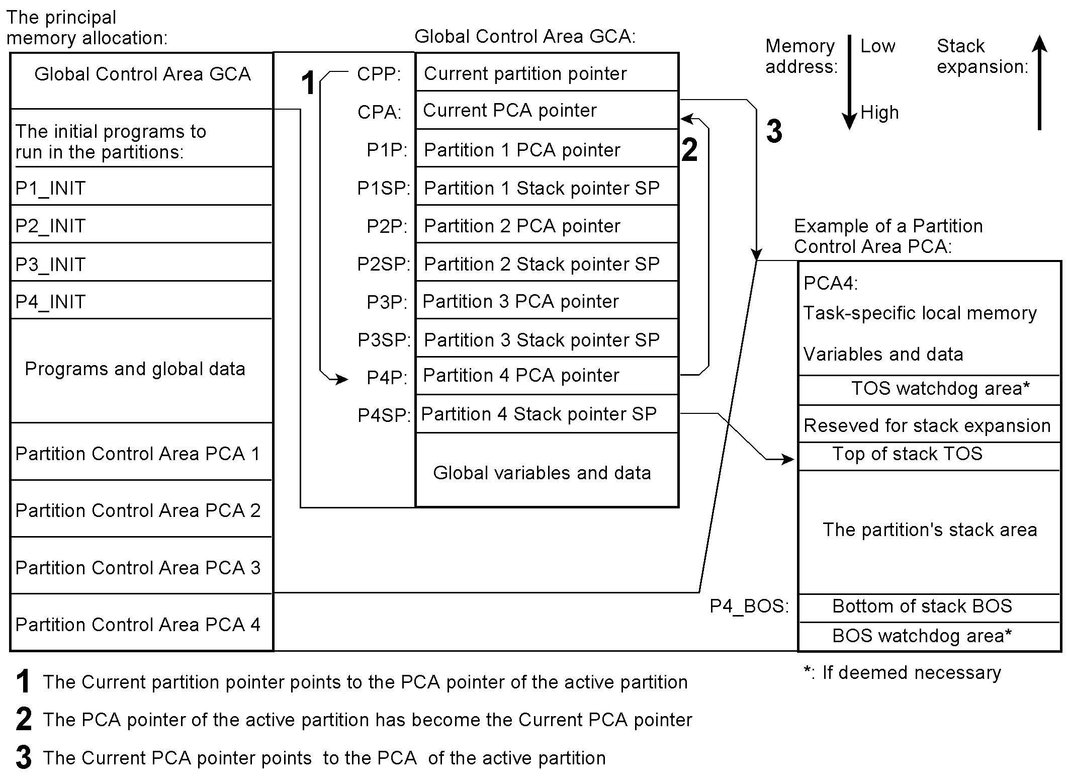
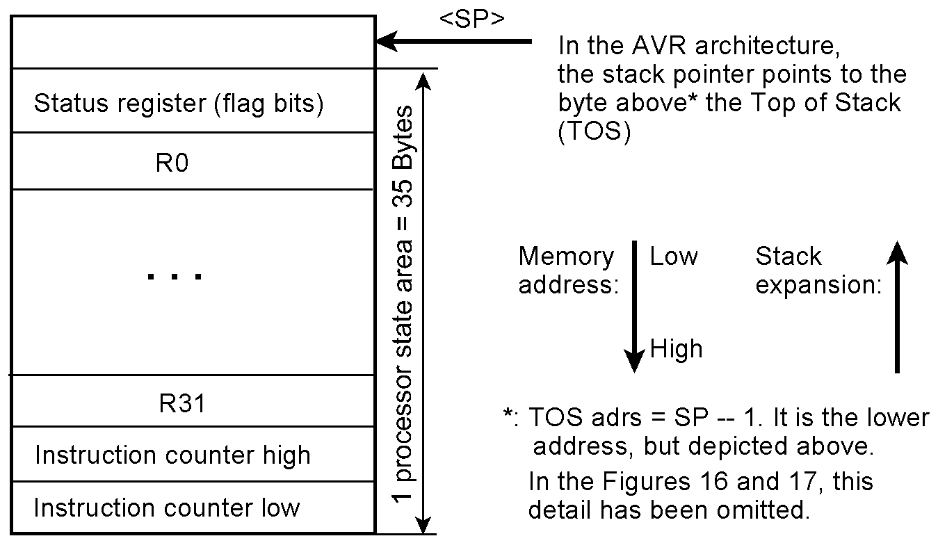
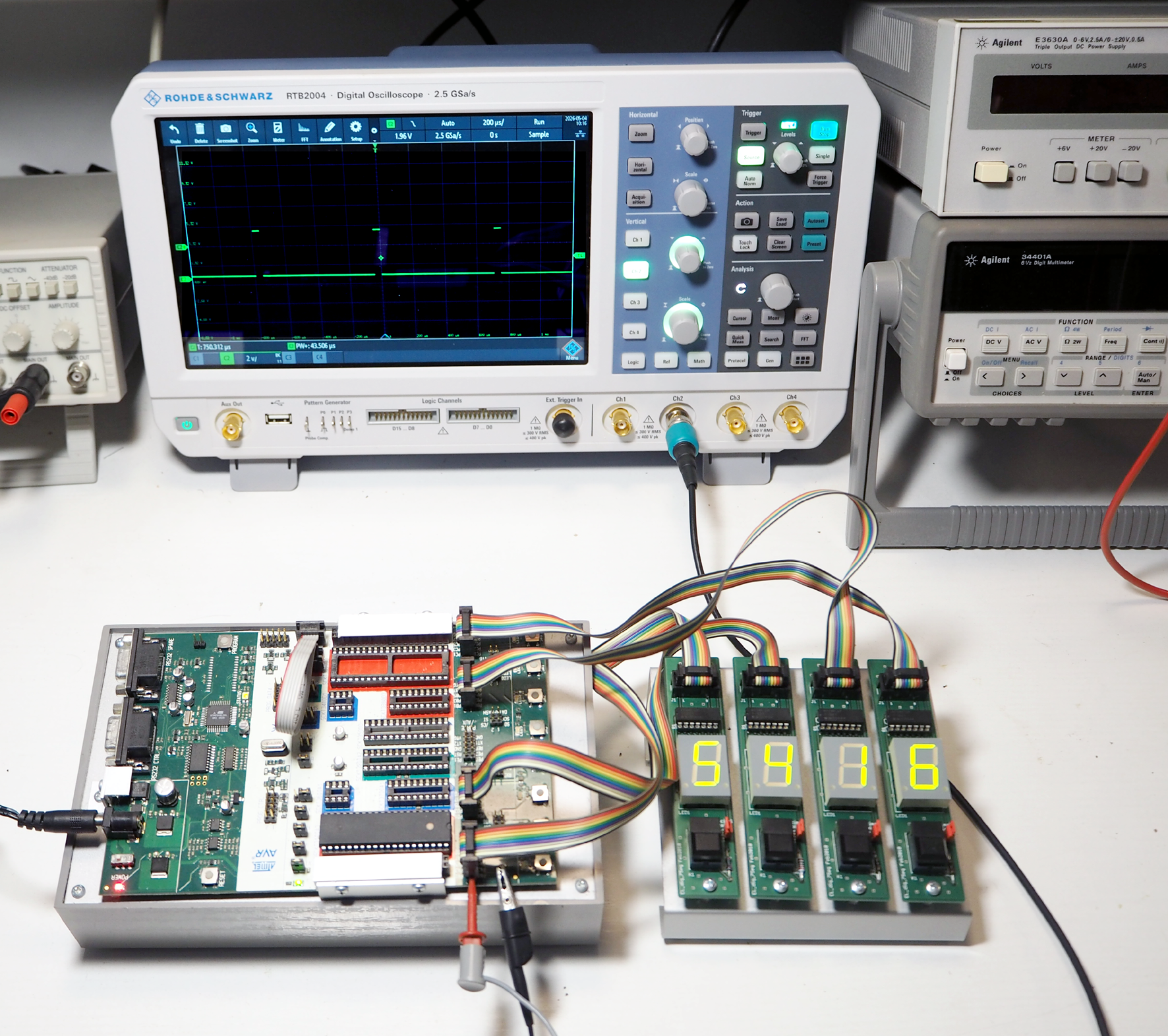
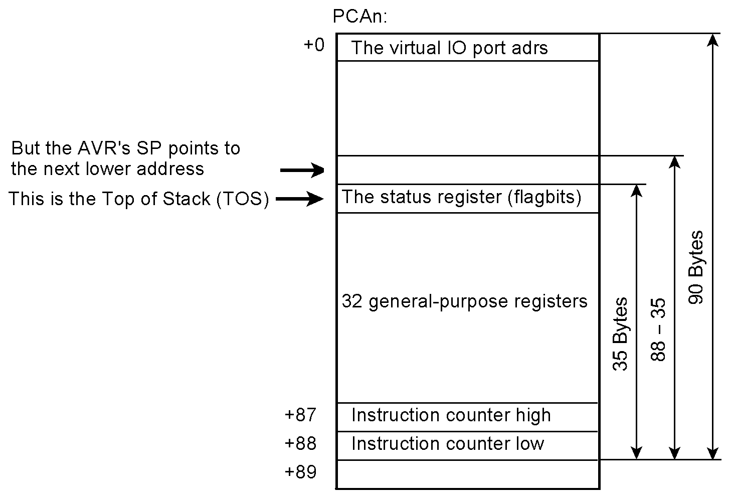
Task switching initiated by a timer interrupt.

The AVR multitasking example
 It has been implemented by straightforward assembler programming. The target processor is the ATmega16. Because the primary objective is task switching, the application should be as simple as possible. Thus, it consists of four basic electronic dice, each implemented by a seven-segment LED display and a key (Figure 18). Each die is connected to one of the I/O ports. Additionally,  I have used bit 0 of I/O port A  to output a pulse to measure the duration of the task swapping and the time slices. The bit is set before the pushes begin and cleared after the pops end.

All dice are supported by only one common application program, which is executed for each die separately. Therefore, the program cannot refer to particular I/O addresses. The problem has been solved by resorting to the port’s memory addresses (Table 2).  In the source code, they are dubbed virtual port addresses.

Each partition control area (PCA) has been assigned 90 bytes. The stack is located at the upper end.  Address calculation to initialize the stack correctly is somewaht tricky, as illustrated in Figure 19.

Figure 18
The platform is an Atmel STK500 starter kit connected to LED display modules of its own design. In the background, the measuring pulses are displayed. With the timing parameter chosen here, task swapping (the pulse duration) is 44 µs: the time slice (the pulse period) is 750 µs. The clock frequency is 4 MHz.

Figure 19
This layout diagram of a Partition Control Area (PCA) explains the mysteries of the address calculation in the assembler program.

Table 2
Accessing the I/O ports via memory addresses (aka virtual port addresses). The PIN addresses are the virtual address parameters.

The source program can be downloaded as avr_example_01.asm. 

May 26, 2026

Download the Internet addendum to the CC article

Download the Internet addendum with the larger figures rotated 90 degrees, so their labelings are easier to read

Download the assembler source program